Geospatial Indexing Explained: A Comparison of Geohash, S2, & H3
Table of Contents
Introduction
Geospatial Indexing is the process of indexing latitude-longitude pairs to small subdivisions of geographical space, and it is a technique that we data scientists often find ourselves using when faced with geospatial data.
While geohash was invented in 2008, governments have subdivided land for centuries using states, provinces, counties, and postal codes for census and electoral purposes.
Data scientists employ computational techniques for spatial subdivision to support:
- Analytics
- Feature-engineering
- Granular AB testing by geographic subdivision
- Indexing geospatial databases
This post examines three tools:
- Geohash
- Google S2
- Uber H3
Note: This article focuses on geospatial indexing functionality specifically, though these tools offer additional capabilities like polygon intersection and neighbor retrieval.
Geohash
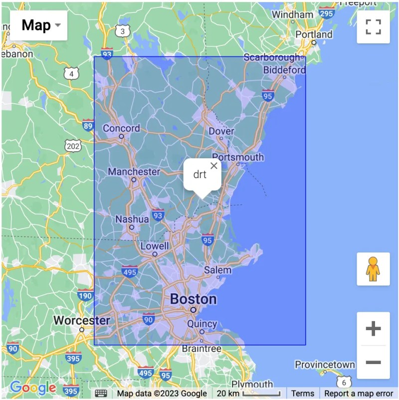
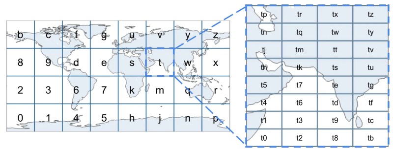
Invented in 2008 by Gustavo Niemeyer, Geohash maps latitude-longitude pairs to squares of user-defined resolution, identified by signature strings like "drt".
The Geohash Algorithm
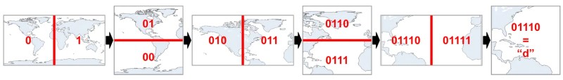
The process involves six steps:
- Choose a geohash-level/resolution
- Create an empty binary array S of length (geohash-level x 5)
- Check if point is in left/right half of map; append 0 or 1 accordingly
- Check if point is in bottom/top half; append 0 or 1 accordingly
- Repeat steps 3-4 (geohash-level x 5 / 2) times
- Convert every 5 bits to a 32-bit alphanumeric character
The algorithm can be repeated iteratively to create increasingly fine-grained divisions, down to cells less than a meter on each side.
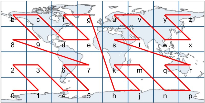
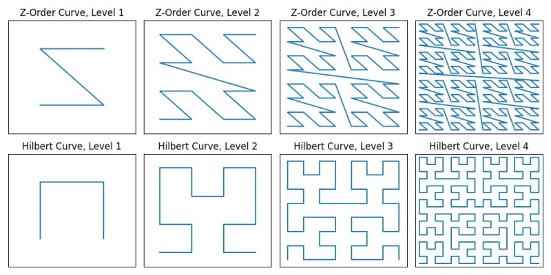
Z-Order Curve
The Z-order curve is a type of space-filling curve, which is designed just for this purpose of mapping multidimensional values (such as latitude-longitude pairs) to one dimensional representations (such as a string).
Alphabetically ordered geohashes trace a Z-order curve pattern.
Geohash's Shortcomings
Problem 1: Weak Spatial Preservation
The Z-order curve weakly preserves latitude-longitude proximity. Due to edge effects, locations physically close may have distant geohash strings, and vice versa — locations with similar hash strings may be physically distant.
Problem 2: Projection Issues
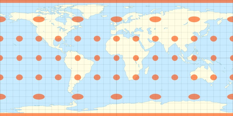
The equirectangular projection creates:
- High variability in geohash square sizes
- Discontinuities at the North and South Poles
Geohashes get smaller as you approach the poles, making the system unreliable at polar regions. Antarctica at (-90°, 0°) cannot be represented.
Getting Started with Geohash
Geohash implementations are widely available:
- PyPi libraries: geohashr, geohash-tools, pygeohash-fast
- Rust crate: Rust-Geohash
- NodeJS library: node-geohash
- Database tools: PostGIS, AWS Redshift, GCP BigQuery
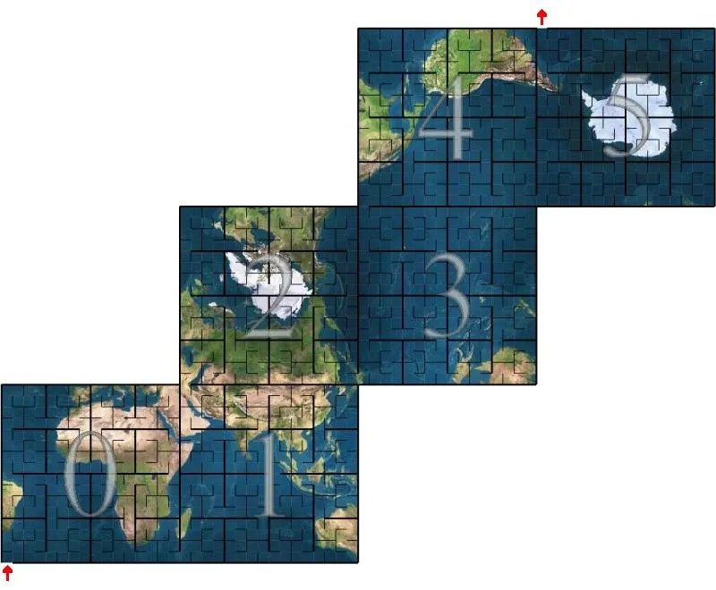
Google S2
Released December 5, 2017, created primarily by Eric Veach at Google. S2 addresses Geohash's limitations through two innovations:
- Hilbert curve (instead of Z-order curve)
- Unfolded cube projection (instead of equirectangular projection)
The Hilbert Curve
The Hilbert curve is another type of space-filling curve that, rather than using a Z-shaped pattern like the Z-order curve, uses a gentler U-shaped pattern.
The Hilbert curve requires more distance to index the same space compared to Z-order curves at all levels. This provides better locality-sensitive hashing properties.
Key advantage: latitude-longitude pairs that are close in their S2 Cell ID string distance are much more likely to be close in physical distance.
Note: Edge effects still exist, but latitude-longitude pairs close in physical distance aren't necessarily close in string distance.
The S2 Map Projection
S2 uses an unfolded-cube projection rather than equirectangular projection. This significantly reduces cell size variation because as you move away from the equator, the distance between two longitude lines increases sinusoidally.
Getting Started with S2
- Primary: C++ implementation on Google's Github
- Ports: Kotlin, Java, Golang
- Alternative: Open-source Python implementation by third parties (aaliddell/s2cell on Github)
Note: Python interface requires non-trivial setup.
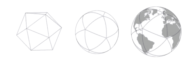
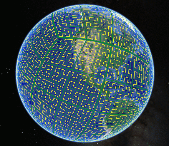
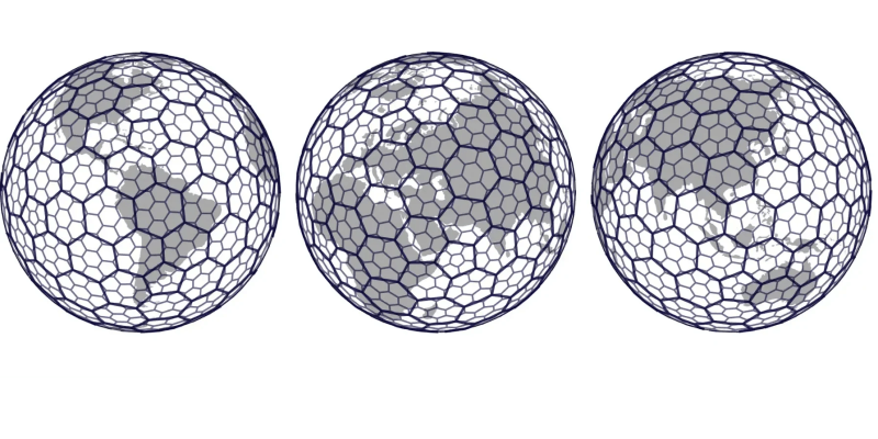
Uber H3
Released 2018, H3 introduces two further innovations:
- Hexagons (instead of squares)
- Icosahedron projection (instead of cube or equirectangular)
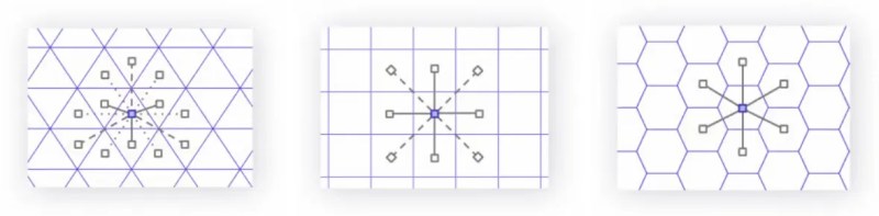
Why Hexagons?
The hexagon is the regular polygon with the most sides that still tessellates with itself.
Key property: In a hexagon tessellation, all neighbors of any hexagon are equidistant from its center.
This differs from:
- Triangles: Three distinct neighbor distances
- Squares: Two distinct neighbor distances
Having this property that all neighbors are equidistant greatly simplifies any calculus or gradient related operations that Uber or H3's other users might want to perform.
Hexagons appear in nature: bee hives, water crystallization (snowflakes), and Saturn's North Pole storm.
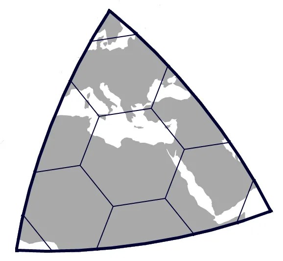
The Icosahedron Projection
H3 uses a 20-faced polyhedron (icosahedron) projected onto Earth. More faces on a polyhedron approximate a sphere more closely, reducing spatial distortion.
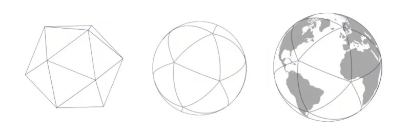
Each triangular face of the icosahedron is covered with hexagons, which subdivide into smaller hexagons from there.
Result: H3 hexagons have more consistent sizes than S2 squares, which have more consistent sizes than Geohash squares.
H3's Sacrifices
Trade-off 1: Hierarchical Structure
Hexagons don't subdivide as cleanly into smaller hexagons. One hexagon divides into seven others, positioned at a slight angle to the parent.
Consequence: the strict spatial hierarchy discussed above regarding Geohash — that if a latitude-longitude point is contained in a cell then it is guaranteed to be contained in that cell's parent — is not maintained in H3.

Example: In Geohash, "h356" is a child of "h35", but in H3, "862830807ffffff" is a child of "85283083fffffff" — string prefixes don't indicate hierarchy.
Trade-off 2: Space-Filling Curve Limitations
While H3 follows a space-filling curve within each icosahedron face, it does not globally. Hexagon string identifiers use a bitmap that doesn't retain string-prefix behavior.
Trade-off 3: Pentagon Necessity
Hexagons cannot perfectly tessellate on a sphere. H3 requires twelve pentagons positioned at icosahedron vertices (like a soccer ball pattern). These are strategically placed over oceans to minimize impact.

Getting Started with H3
- Primary: C implementation on Uber's Github
- Bindings: Python (h3-py), R (h3r), and many other languages
- Availability: Better cross-platform support than S2, though less universal than Geohash
Comparison
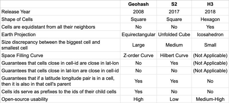
| Criterion | Geohash | S2 | H3 | |-----------|---------|----|----| | Cell Shape | Squares | Squares | Hexagons | | Space-Filling Curve | Z-order | Hilbert | None (icosahedron-based) | | Projection | Equirectangular | Cube | Icosahedron | | Cell Size Consistency | Poor | Good | Excellent | | String Proximity = Physical Proximity | Weak | Better | N/A | | Spatial Hierarchy | Strict | Strict | Approximate | | Availability | Ubiquitous | Limited | Moderate | | Complexity | Simple | Moderate | High |
When to Use Which Tool?
Feature Engineering with Latitude and Longitude
Simple neighborhood ID creation: Any tool works.
Aggregation features (e.g., average lifespan by neighborhood): Any tool functions.
Population density estimation: H3 preferred due to uniform cell sizes.
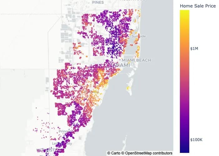
Small geographic areas (e.g., Manhattan): Geohash acceptable to leverage simplicity without distortion effects.
Multiple cell sizes simultaneously: Avoid H3 (creates multiple cell overlap). Choose Geohash or S2.
Ocean-related data: Avoid H3 to prevent pentagon complications.
Conclusion
As our need for richer features from our systems increase, design complexity increases, and with it, so increase the sacrifices we must make regarding the system's properties.
Each tool represents design trade-offs. The analogy is made to digital vs. analog calendars — there's no universally "correct" answer, only context-appropriate choices.
References
Discover How We Can Turn Your Data Into Your Competitive Edge.
We specialize in transforming raw data into strategic value through AI, automation, and analytics.
Chat With Us